The Logical Storage Manager (LSM) software is an optional integrated, host-based disk storage management application that lets you manage storage devices without disrupting users or applications accessing data on those storage devices. Although any system can benefit from LSM, it is especially suited to configurations with large numbers of disks or configurations that regularly add storage.
LSM uses Redundant Arrays of Independent Disks (RAID) technology to enable you to configure storage devices into a virtual pool of storage from which you create LSM volumes. You can configure new and existing UFS and AdvFS file systems, databases, and applications to use LSM volumes. You can also create LSM volumes on top of RAID storage sets.
The benefits of using an LSM volume instead of a disk partition include:
Data loss protection, through mirroring (RAID 1) or striping with parity (RAID5)
Maximized disk usage, by seamlessly combining storage devices to appear as a single storage device to users and applications
Performance improvements, through striping (RAID 0) over different disks and different buses
Data availability in a TruCluster Server environment
TruCluster Server software makes multiple Tru64 UNIX systems appear as a single system on the network. The systems running the TruCluster Server software become members of the cluster and share resources and data storage. This sharing allows applications, such as LSM, to continue uninterrupted if the cluster member on which it was running fails.
This chapter introduces LSM features, concepts, terminology, and available
interfaces.
For more information on LSM terms and a list of all the LSM commands,
see
volintro(8)1.1 Overview of the LSM Object Hierarchy
LSM uses the following hierarchy of objects to organize storage:
LSM disk — An object that represents a storage device that is initialized exclusively for use by LSM
Disk Group — An object that represents a collection of LSM disks for use by an LSM volume
Subdisk — An object that represents a contiguous set of blocks on an LSM disk that LSM uses to write volume data
Plex — An object that represents a subdisk or collection of subdisks to which LSM writes a copy of the volume data or log information
Volume — An object that represents a hierarchy of LSM objects, including LSM disks, subdisks, and plexes in a disk group. Applications and file systems make read and write requests to the LSM volume.
The following sections describe LSM objects in more detail.
1.1.1 LSM Disk
An LSM disk is any storage device supported by Tru64 UNIX, including disks, disk partitions, and hardware RAID sets, that you configure exclusively for use by LSM. LSM views the storage in the same way as the Tru64 UNIX operating system software views it. For example, if the operating system software treats a RAID set as a single storage device, so does LSM. In addition, LSM recognizes and supports hardware disk clones.
For more information on supported storage devices, see the Tru64 UNIX QuickSpecs web site at the following URL:
http://www.tru64unix.compaq.com/docs/pub_page/spds.html
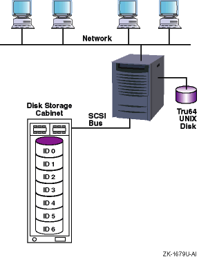
Figure 1-1
shows a typical hardware configuration that LSM
supports.
Figure 1-1: Typical LSM Hardware Configuration
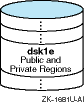
A storage device becomes one of the following LSM disk types when you initialize it for use by LSM:
A sliced disk, which is created when you commit an entire disk to LSM use.
In a
sliced
disk, LSM organizes the storage into
two regions on separate partitions — a large
public region
used for storing data and a
private region
for storing LSM internal metadata, such
as LSM configuration information.
The default size of the private region is
4096 blocks.
A
simple disk, which
is created when you specify a disk partition for LSM use, including the
c
partition.
In a
simple
disk, LSM organizes the storage into
two regions on the same partition — a large public region used for storing
data and a private region for storing LSM internal metadata, such as LSM configuration
information.
The default size of the private region is 4096 blocks.
Whenever possible, initialize the entire disk as a
sliced
disk instead of configuring individual disk partitions as
simple
disks.
This ensures that the disk's storage is used efficiently
and avoids using space for multiple private regions on the same disk.
A nopriv disk, which is created when you encapsulate a disk or disk partition containing data you want to place under LSM control.
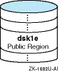
In a
nopriv
disk, LSM creates only a public region
for the existing data and no private region.
When you initialize a disk for LSM use, LSM assigns it a
disk access name
based on the device you specify.
For example,
if you initialize an entire disk (for example,
dsk4), the
disk access name is
dsk4.
If you initialize a disk partition
(for example,
dsk4b), the disk access name is
dsk4b.
If you initialize multiple partitions of the same disk as separate LSM
disks, each has its own disk access name; for example,
dsk2b
and
dsk2f.
1.1.1.2 Disk Media Name
When you add an LSM disk to a disk group, it gets a disk media name, which can be either the same as the disk access name or a name you assign. Disk media names can include any combination of up through 31 alphanumeric characters but cannot include spaces or a slash ( / ).
For example, a disk with a disk access name of
dsk1
can also have a disk media name of
dsk1
or a name you assign,
such as
finance_data_disk.
LSM keeps track of the association of the disk media name and the disk access name. The disk media name provides insulation from operating system naming conventions. This association allows LSM to find the device if you move it to a new location (for example, to a different controller).
If you remove a disk from a disk group, it loses its disk media name. If you add the disk to a different disk group you can give it a different disk media name, or let it use the disk access name by default.
Within a disk group all the disk media names must be unique, but two
different disk groups can have disks with the same disk media name.
1.1.2 Disk Group
A
disk group
is an object that represents a grouping of LSM disks.
LSM disks in a disk
group share a common
configuration
database
that identifies all the LSM objects (LSM disks,
subdisks, plexes, and volumes) in the disk group.
LSM automatically creates
and maintains copies of the configuration database in the private region of
several LSM
sliced
or
simple
disks in
each disk group.
The default size of the private region is 4096 blocks, and each LSM object requires one record. Two records fit in one sector (512 bytes). Therefore, the default private region size guarantees space for a configuration database that tracks 8192 objects (LSM disks, subdisks, plexes, and volumes).
LSM distributes these copies across all controllers for redundancy. If all disks in a disk group are located on the same controller, LSM distributes the copies across several disks. LSM automatically records changes to the LSM configuration and, if necessary, changes the number and location of copies of the configuration database for a disk group.
You cannot have a disk group that contains only LSM
nopriv
disks, because an LSM
nopriv
disk does not have
a private region to store copies of the configuration database.
By default, the LSM software creates a disk group named
rootdg.
The configuration database for
rootdg
contains information for itself and all other disk groups that
you create.
An LSM volume can use disks only within the same disk group.
You can
create all of your volumes in the
rootdg
disk group, or
you can create other disk groups.
For example, if you dedicate disks to store
financial data, you can create and assign those disks to a disk group named
finance.
1.1.3 Subdisk
A subdisk is an object that represents a contiguous set of blocks in an LSM disk's public region that LSM uses to store data.
By default, LSM assigns subdisk names using the LSM disk media name
followed by a dash (-) and an ascending two-digit number beginning with
01; for example,
dsk1-01.
Alternatively, you can assign a subdisk name of up to 31 alphanumeric
characters that cannot include spaces or the slash ( / ).
For example, you
can assign a subdisk name of
finance_disk-01
on a disk
with a disk media name of
dsk3.
A subdisk can be:
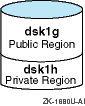
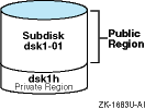
The
entire public region.
Figure 1-2
shows that the entire public region of an LSM disk
was configured as a subdisk named
dsk1-01.
Figure 1-2: Single Subdisk Using a Public Region
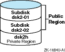
A
portion of the public region.
Figure 1-3
shows a public region of an LSM disk that was configured
as two subdisks named
dsk2-01
and
dsk2-02.
Figure 1-3: Multiple Subdisks Using a Public Region
A data plex is an object that represents a subdisk or collection of subdisks in the same disk group to which LSM writes volume data.
By default, LSM assigns plex names using the volume name followed by
a dash (-) and an ascending two-digit number beginning with 01.
For
example,
volume1-01
is the name of the first (or only)
plex in a volume named
volume1.
Alternatively, you can assign a plex name of up to 31 alphanumeric characters
that cannot include spaces or the slash ( / ).
For example, you can assign
a plex name of
finance_plex01.
You can use one of three types of data plex depending on how you want LSM to store volume data on disk:
In a concatenated data plex, LSM writes volume data in a linear manner. When the space in one subdisk has been written to, the remaining data goes to the next sequential subdisk in the plex. Section 1.1.4.1 explains this plex type in more detail. A volume can contain two or more concatenated data plexes, in which case the volume is described as concatenated and mirrored.
In a striped data plex, LSM separates data into equal-sized data units (defined by the stripe width) and writes the data units to each disk in the plex. This attempts to balance the load across all disks. Section 1.1.4.2 explains this plex type in more detail. A volume can contain two or more striped data plexes, in which case the volume is described as striped and mirrored.
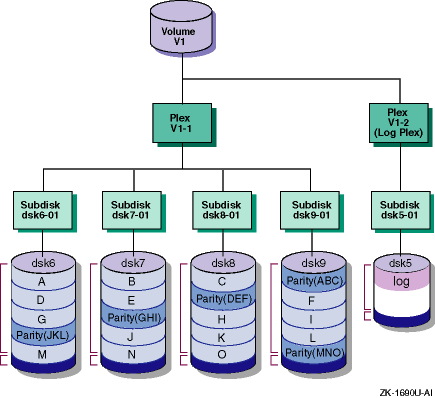
In a RAID5 data plex, LSM calculates a parity value for the data being written, then separates the data and parity into equal-sized data units (defined by the stripe width), and intersperses the data and parity across all disks. Section 1.1.4.3 explains this plex type in more detail. A volume can contain only one RAID5 data plex, due to internal design constraints.
1.1.4.1 Concatenated Data Plex
In a concatenated data plex, LSM creates a contiguous address space
on the subdisks and sequentially writes volume data in a linear manner.
If
LSM reaches the end of a subdisk while writing data, it continues to write
data to the next subdisk, which might be on a different physical disk (Figure 1-4).
LSM lets you use space on several disks that otherwise
might be unusable.
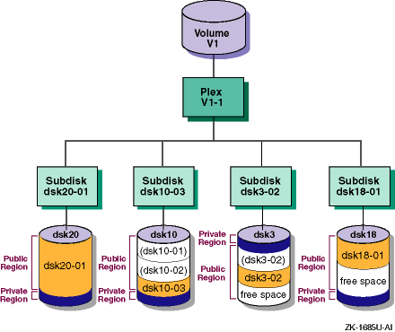
One disk's public region can contain subdisks used in several
different volumes.
Figure 1-4: Concatenated Data Plex
A single subdisk failure in a volume with one concatenated data plex will result in LSM volume failure. To prevent this type of failure, you can create multiple plexes (mirrors) on different disks. LSM continuously maintains the data in the mirrors. If a plex becomes unavailable because of a disk failure, the volume continues operating using another plex.
Using disks on different SCSI buses for mirror plexes speeds read requests,
because data can be simultaneously read from multiple plexes.
1.1.4.2 Striped Data Plex
In a striped data plex, LSM divides a write request into equal-size data units, defined by the stripe width (64K bytes by default) and writes each data unit to a different disk, creating a stripe of data across the columns (usually, the number of disks in the plex). You can define a different stripe width (data unit size) to achieve the best division of data across the columns.
LSM can simultaneously write two or more data units if the disks are on different SCSI buses.
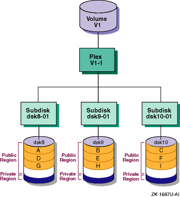
Figure 1-5
shows a three-column striped plex.
In this type of plex, an I/O write request is divided into equal-size units
(A, B, C, D, and so on) and each data unit is written sequentially to a different
subdisk (in a different disk column).
Figure 1-5: Volume with a Three-Column Striped Data Plex
If a write request does not complete a stripe (the number of data units is not evenly divisible by the number of columns), then the first data unit of the next write request starts in the next column.
If a write request is not evenly divisible by the data unit size, so that the last data unit in a write request does not map to the end of a column, the next write request completes the column then continues to subsequent columns.
As in a concatenated data plex, a single disk failure in a volume with one striped data plex will result in volume failure. To prevent this type of failure, you can create multiple data plexes (mirrors) on different disks. LSM continuously maintains the data in the mirrored data plexes. If a plex becomes unavailable because of a disk failure, the volume continues operating using another plex.
Using disks on different SCSI buses for mirror plexes speeds read requests,
because data can be simultaneously read from multiple plexes.
1.1.4.3 RAID 5 Data Plex
In a RAID 5 data plex, LSM calculates a parity value for each stripe of data, then separates the data and parity into equal-size units defined by the stripe width (16K bytes by default) and writes the data and parity units on three or more columns of subdisks, creating a stripe of data and parity across the columns. The parity is contained in one data unit to ensure that each column of disks contains the entire parity value for any given data stripe.
LSM writes the parity in a different column for each consecutive stripe of data. The parity unit for the first stripe is written to the last column. Each successive parity unit is located in the next column to the left of the previous parity unit location. If there are more stripes than columns, the parity unit placement begins again in the last column.
If a disk in one column fails, LSM continues operating using the data and parity information in the remaining columns to reconstruct the missing data. You can define a different stripe width (data unit size) to achieve the best division of data and parity across the columns.
LSM can simultaneously write the data and parity units if the columns are on different SCSI buses.
Figure 1-6
shows how data and parity information are
written in a RAID5 data plex.
Figure 1-6: Volume with a RAID 5 Data Plex
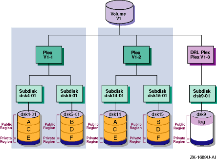
A log plex contains information about activity in a volume. After a system failure, LSM recovers only those areas of the volume identified in the log plex as being dirty (written to) at the time of the failure.
By default, LSM creates a log plex for mirrored volumes (volumes with two or more striped or concatenated data plexes) and for volumes that use a RAID5 data plex. Mirrored volumes use a Dirty Region Log (DRL) plex and an optional Fast Plex Attach (FPA) plex. RAID5 volumes use a RAID5 log plex.
In a DRL plex, LSM keeps track of the regions of a volume that change due to I/O requests. When the system restarts after a crash, LSM resynchronizes only the regions marked as dirty in the log. This greatly reduces the time needed to resynchronize the volume, especially for volumes of hundreds of megabytes or more.
Regions are marked as dirty before the data is written. When the write completes, the region is not immediately marked as clean but instead allowed to stay dirty for a specific length of time. This reduces the overhead of marking the log if another write occurs to the same region. If a dirty region has had no activity for an extended period of time, it is marked as clean.
If you do not use a DRL plex, LSM copies and resynchronizes all the data to each plex to restore the plex consistency when the system restarts after a failure. Although this process occurs in the background and the volume is still available, it can be a lengthy procedure and can result in unnecessarily recovering data, thereby degrading system performance.
Fast Plex Attach (FPA) log plex
A Fast Plex Attach log plex is used to support backups of mirrored volumes. An FPA log tracks the regions of a volume that change while one of its data plexes is detached. The detached plex is used to create a secondary volume for performing backups. When the plex returns to the original volume, only the regions marked in the FPA log plex are written to the returning plex, reducing the time required to resynchronize that plex to the volume.
In a RAID5 log plex, LSM stores a copy of the data and parity for several full stripes of I/O. When a write to a RAID5 volume occurs, the parity is calculated and the data and parity are first written to the RAID5 log, then to the volume. When the system is restarted after a crash, all the writes in the RAID5 log are written (or possibly rewritten) to the volume. The RAID5 log plex uses a special log subdisk.
In addition, for compatibility with Version 4.0, LSM supports a combination
data and log plex.
This type of plex is not used in Version 5.0 and higher.
1.1.6 LSM Volume
A volume is an object that represents a hierarchy of plexes, subdisks, and LSM disks in a disk group. Applications and file systems make read and write requests to the LSM volume. The LSM volume depends on the underlying LSM objects to satisfy the request.
An LSM volume can use storage from only one disk group.
LSM does not assign default names to volumes; you must assign a name of up to 31 alphanumeric characters that does not include spaces or the slash ( / ). Within a disk group the volume names must be unique, but two different disk groups can have volumes with the same name.
LSM volumes can be either redundant or nonredundant.
A redundant volume
provides high data availability, either through mirroring (two or more concatenated
or striped data plexes) or through parity (RAID5 data plex).
The following sections describe these properties in more detail.
1.1.6.1 Nonredundant Volumes
A nonredundant volume has one data plex and therefore does not provide any data redundancy. The plex layout can be either striped or concatenated.
A nonredundant volume with one concatenated plex is called a
simple volume, which can comprise space on one or more disks.
This
is the simplest volume type.
A simple volume usually has the slowest performance
of all the volume types.
1.1.6.2 Mirrored Volumes
A mirrored volume has two or more data plexes, which are either concatenated or striped, and a log plex (by default). Depending on the plex layout, this type of volume is also called a concatenated and mirrored volume or a striped and mirrored volume. Usually, all the data plexes in a volume have the same layout (all striped or all concatenated), but this is not a restriction.
Each data plex is an instance of the volume data. A mirrored volume provides data redundancy and improved read performance, as data can be read from any mirror. Mirrored volumes can have up to 32 plexes in any combination of data and DRL plexes, but by definition mirrored volumes have at least two data plexes. Mirrored volumes are redundant volumes, because each mirror (plex) contains a complete copy of the volume data.
Figure 1-7
shows a volume with concatenated
and mirrored data plexes and a Dirty Region Log (DRL) plex (Section 1.1.5).
Figure 1-7: Volume with Concatenated and Mirrored Data Plexes
Figure 1-8
shows a volume with striped
and mirrored data plexes and a DRL plex.
Figure 1-8: Volume with Striped and Mirrored Data Plexes
Different LSM volumes can use disk space on the same disk, but in different
subdisks.
Figure 1-9: Two LSM Volumes Using Subdisks on the Same Disk
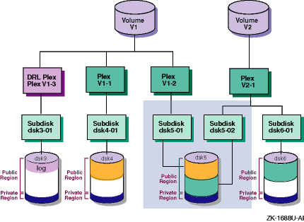
In
Figure 1-9, volume
V1
uses space on disk
dsk5
in subdisk
dsk5-01.
Volume
V2
uses space on disk
dsk5
as
well, but in subdisk
dsk5-02.
Volume
V1
is striped and mirrored (uses two striped
plexes), and volume
V2
is a simple volume (uses one concatenated
plex).
If disk
dsk5
fails, volume
V1
continues running using plex
V1-1.
However, volume
V2
will fail completely because it is not redundant.
1.1.6.3 RAID 5 Volumes
A RAID 5 volume has one RAID5 data plex and one RAID5 log plex. You can add multiple RAID5 log plexes to the volume, but one is sufficient. RAID5 volumes are redundant volumes, because the volume preserves data redundancy through the parity information.
Note
You cannot mirror a RAID 5 data plex.
The TruCluster Server software does not support RAID5 volumes.
An LSM volume has a usage type that defines a particular class of rules for operating on the volume. The rules are typically based on the expected content of the volume. The LSM usage types include:
fsgen
— For volumes that contain
file systems.
This is the default usage type.
gen
— For volumes used for swap space
or other applications that do not use the system buffer cache (such as a database).
raid5
— For all RAID5
volumes, regardless of what the volume contains.
In addition, LSM uses the following special usage types:
root
— For the
rootvol
volume, created by encapsulating the root partition on a standalone system.
swap
— For the primary swap volume,
created by encapsulating the primary swap partition on a standalone system.
For the swap volumes of cluster members, created by encapsulating the members'
swap devices.
cluroot
— For the
cluster_rootvol
volume, created by migrating the clusterwide root file system domain
to an LSM volume in a TruCluster Server cluster.
1.1.6.5 Volume Device Interfaces
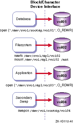
Like most storage devices, an LSM volume has a block device interface and a character device interface.
A volume's block device interface is located in the
/dev/vol/disk_group
directory.
A volume's character device interface is located in the
/dev/rvol/disk_group
directory.
Databases, file systems, applications, and secondary swap use an LSM
volume in the same manner as a disk partition because these interfaces support
the standard UNIX
open,
close,
read,
write, and
ioctl
calls
(Figure 1-10).
Figure 1-10: LSM Volumes Used Like Disk Partitions
1.2 Overview of LSM Interfaces
You can create, display, and manage LSM objects using one of the following interfaces:
A command-line interpreter (CLI), where you enter LSM commands at the system prompt. This manual focuses chiefly on LSM CLI commands.
The CLI provides the full functionality of LSM. The other interfaces might not support some LSM operations.
A Java-based graphical user interface (GUI) called LSM Storage
Administrator (lsmsa) that displays a hierarchical view
of LSM objects and their relationships.
A menu-based, interactive interface called
voldiskadm
that supports a limited number of LSM operations on disks and disk
groups.
To perform a procedure through the
voldiskadm
interface,
you choose an operation from the main menu and the interface prompts you for
information.
The
voldiskadm
interface provides default
values when possible.
You can press Return to use the default value or enter
a new value or enter
?
at any time to view online help.
For more information, see
voldiskadm(8)
A bit-mapped GUI called Visual Administrator (dxlsm) that uses the Basic X Environment.
The Visual Administrator lets you view and manage disks and volumes and perform limited file system administration. The Visual Administrator displays windows in which LSM objects are represented as icons.
Note
The Visual Adminstrator (
dxlsm) has been replaced by the Storage Administrator (lsmsa).
For more information, see
dxlsm(8X)
In many cases, you can use the LSM interfaces interchangeably.
That
is, LSM objects created by one interface are usually manageable through and
compatible with LSM objects created by other LSM interfaces; however, the
Fast Plex Attach feature is available only through the CLI.
1.2.1 LSM Command-Line Interpreter
The LSM command-line interpreter provides you with most control and
specificity in creating and managing LSM objects.
The other interfaces (lsmsa,
voldiskadm, and
dxlsm)
do not support all the operations available through the command line.
Most LSM commands fall into two categories: high-level and low-level.
The high-level commands are generally more powerful than the low-level commands and are the recommended method of performing the majority of LSM operations. The high-level commands are shortcuts; they might pass the specified operands or values to several low-level commands, initiating many operations with just one command. The high-level commands sequence the intermediate steps in the correct order and also perform a certain amount of error checking by evaluating the operands you specify and the intended end result of the operation, alerting you to problems. The high-level commands use algorithms and default values that provide the best LSM configuration for the majority of cases.
This manual focuses chiefly on the high-level LSM commands, except where more specificity than they provide is required.
The low-level commands require detailed knowledge and understanding of your particular environment and what you are trying to achieve with your LSM configuration. The low-level commands operate on specific LSM object types. In many cases you must perform several operations, sometimes in a precise order, to accomplish what the high-level commands can do for you in fewer steps and with less risk of error.
Table 1-1 lists the LSM commands described in this manual, their functions, and, where applicable, indicates whether the command is considered a high-level or low-level command.
Table 1-1: LSM Commands Described in This Manual
| Command | Function | Command Level (If Applicable) |
| Setup and Daemon Commands | ||
volsetup |
Initializes the LSM
software by creating the
|
— |
volsave |
Backs up the LSM configuration database. |
— |
volrestore |
Restores the LSM configuration database. |
— |
voldctl,
vold,
voliod |
Controls LSM volume configuration and kernel daemon operations. |
— |
volwatch |
Monitors LSM for failure events and performs hot-sparing if enabled. Used typically only during initial LSM setup to enable the hot-sparing feature. |
— |
| Object Creation and Management Commands | ||
volassist |
Creates, mirrors, backs up, and moves volumes automatically. |
High-level — The most-often used LSM command for creating and managing LSM volumes. |
voldiskadd |
Creates LSM disks and disk groups. |
High-level — Performs many of the same functions
as
voldisksetup
and
voldg, in one interactive
session |
voldisksetup |
Adds one or more disks for use with LSM. |
High-level |
voldisk |
Administers LSM disks. |
Low-level |
voldg |
Administers disk groups. |
High-level |
volume |
Administers volumes. |
Low-level |
volplex |
Administers plexes. |
Low-level |
volsd |
Administers subdisks. |
Low-level |
volmake |
Creates LSM objects manually. |
Low-level |
voledit |
Creates, modifies, and removes LSM records. |
Low-level |
volrecover |
Synchronizes plexes and parity data after a crash or disk failure. |
High-level |
volmend |
Mends simple problems in configuration records. |
Low-level |
volevac |
Evacuates all volume data from a disk. |
High-level |
| Data Migration and Encapsulation Commands | ||
volencap |
Sets up scripts to encapsulate disks or disk partitions to LSM volumes. |
— |
volreconfig |
Performs the encapsulation scripts set up by
|
— |
volrootmir |
Mirrors the root and swap volumes. (Not supported in a cluster.) |
— |
volunroot |
Removes the root and swap volumes. (Not supported in a cluster.) |
— |
volmigrate,
volunmigrate |
Migrates AdvFS domains to or from LSM volumes. |
— |
vollogcnvt |
Converts volumes with Block Change Logging (pre-Version 5.0) to Dirty Region Logging (Version 5.0 and higher). |
— |
| Informational Commands | ||
volprint |
Displays LSM configuration information. |
— |
voldisk |
Displays information about LSM disks. |
— |
volinfo |
Displays volume status information. |
— |
volstat |
Displays LSM statistics. |
— |
volnotify |
Displays LSM configuration events. |
— |
| Interface Start-Up Commands | ||
lsmsa |
Starts the LSM Storage Administrator GUI. |
— |
In addition to commands, LSM includes the
volmake(4)vol_pattern(4)
For more information on a command, see the reference page corresponding
to its name.
For example, for more information on the
volassist
command, enter:
# man volassist
For a list of LSM commands and files, see
volintro(8)1.2.2 Storage Administrator Interface
The Storage Administrator provides dialog boxes in which you enter information to create or manage LSM objects. Completing a dialog box can be the equivalent of entering several commands. The Storage Administrator lets you manage local or remote systems on which LSM is running. You need an LSM license to use the Storage Administrator.
For more information, see Appendix A.